#basic imports
import os
import tensorflow as tf
from tensorflow.keras import utils
import tensorflow.keras.layers as layers
from matplotlib import pyplot as pltIn this tutorial we’ll be using Tensorflow to create a neural network that can classify images of cats and dogs. These are the imports we’ll be using, both for the neural network and for plotting our results.
Next, we need to import the data we’ll be using to train, validate, and test our neural network. In other words, we need thousands of pictures of cats and dogs! From the validation dataset we take every fifth image to use as a testing dataset at the end of the process. Note also that we have some global parameters for the datasets. The data is split into batches of 32, and each image is 160x160 pixels.
# location of data
_URL = 'https://storage.googleapis.com/mledu-datasets/cats_and_dogs_filtered.zip'

# download the data and extract it
path_to_zip = utils.get_file('cats_and_dogs.zip', origin=_URL, extract=True)

# construct paths
PATH = os.path.join(os.path.dirname(path_to_zip), 'cats_and_dogs_filtered')

train_dir = os.path.join(PATH, 'train')
validation_dir = os.path.join(PATH, 'validation')

# parameters for datasets
BATCH_SIZE = 32
IMG_SIZE = (160, 160)

# construct train and validation datasets
train_dataset = utils.image_dataset_from_directory(train_dir,
                                                   shuffle=True,
                                                   batch_size=BATCH_SIZE,
                                                   image_size=IMG_SIZE)

validation_dataset = utils.image_dataset_from_directory(validation_dir,
                                                        shuffle=True,
                                                        batch_size=BATCH_SIZE,
                                                        image_size=IMG_SIZE)

# construct the test dataset by taking every 5th observation out of the validation dataset
val_batches = tf.data.experimental.cardinality(validation_dataset)
test_dataset = validation_dataset.take(val_batches // 5)
validation_dataset = validation_dataset.skip(val_batches // 5)
Downloading data from https://storage.googleapis.com/mledu-datasets/cats_and_dogs_filtered.zip
68606236/68606236 [==============================] - 2s 0us/step
Found 2000 files belonging to 2 classes.
Found 1000 files belonging to 2 classes.The following code is not necessary, but helps us with reading our data more quickly.
AUTOTUNE = tf.data.AUTOTUNE

train_dataset = train_dataset.prefetch(buffer_size=AUTOTUNE)
validation_dataset = validation_dataset.prefetch(buffer_size=AUTOTUNE)
test_dataset = test_dataset.prefetch(buffer_size=AUTOTUNE)
Before we begin making models, let’s see a few examples of the images that we have.
class_names = ["cat","dog"]

def visualize():
  fig = plt.figure(figsize=(10, 10))
  count = [0,0]
  for images,labels in train_dataset.take(1):
    #takes one batch of images; we assume that the batch contains at least 3 cat and 3 dog pictures
    i = 0
    while (min(count) < 3): #terminates when we have 3 of each animal picture displayed
      if count[labels[i].numpy()] < 3:
        #show ith image in respective axis if there are not already enough images of the same animal
        ax = plt.subplot(2, 3, 3*labels[i].numpy()+count[labels[i]]+1)
        plt.imshow(images[i].numpy().astype("uint8"))
        plt.title(class_names[labels[i]])
        plt.axis("off")
        count[labels[i]] += 1
      i += 1
  return fig

visualize().show()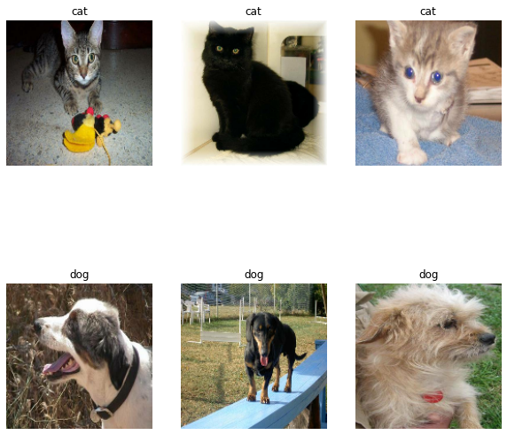
It’s easy for a human to tell the difference between a cat and a dog in these images, but it’s hard to fathom how a computer might do the same. For reference, let’s see how many images of each type of animal we have.
labels_iterator= train_dataset.unbatch().map(lambda image, label: label).as_numpy_iterator()
labels = [i for i in labels_iterator]
num_dogs = sum(labels)
num_cats = len(labels)-num_dogs
(num_cats,num_dogs)
WARNING:tensorflow:From /usr/local/lib/python3.8/dist-packages/tensorflow/python/autograph/pyct/static_analysis/liveness.py:83: Analyzer.lamba_check (from tensorflow.python.autograph.pyct.static_analysis.liveness) is deprecated and will be removed after 2023-09-23.
Instructions for updating:
Lambda fuctions will be no more assumed to be used in the statement where they are used, or at least in the same block. https://github.com/tensorflow/tensorflow/issues/56089(1000, 1000)A baseline image classification model should guess “cat” or “dog” with 50% probability each, since there are an equal number of each label. In this case the model accuracy would be 50%, since the guess is not correlated with the given image.
##Model 1
Now let’s actually make a machine learning model. A neural network consists of a sequence of layers that feed into each other linearly. Each layer takes in a tensor as input, performs some sort of analysis on it, and outputs another tensor. In Tensorflow, this is implemented using the Sequential object, which takes in a list of layers from tensorflow.keras.layers.
#creates model as a Sequential object
model1 = tf.keras.models.Sequential([
    layers.Conv2D(2,3, input_shape=(160,160,3)),
    layers.MaxPooling2D(),
    layers.Dropout(rate=0.1),
    layers.Conv2D(2,3, input_shape=(80,80,3)),
    layers.MaxPooling2D(),
    layers.Dropout(rate=0.1),
    layers.Flatten(),
    layers.Dense(2, activation='softmax'),
])
This first model we created has five different types of layers:
Conv2Dperforms 2-dimensional convolution on the input data. The first parameter is the number of output filters, and the second parameter is the kernel size of the convolution.MaxPooling2Dpools input data by choosing the maximum value in each block of a given size (by default(2,2)).Dropoutrandomly changes input values to 0 at therateprovided. This helps prevent overfitting.Flattenreshapes the input tensor into a 1-dimensional tensor.Denseis a densely connected layer, which means that it takes in every entry in the previous layer as input and performs linear algebra on it. The first parameter indicates the dimensionality of the output space, and theactivationparameter indicates the type of activation function we want to use.
Next, we compile and train our model. We use Adam optimization, which is a stochastic gradient descent method, and our loss function is calculated in terms of cross entropy. For the purposes of this assignment, we’ll always be training with 20 epochs.
#compile model1
sce = tf.keras.losses.SparseCategoricalCrossentropy(from_logits=False)

model1.compile(optimizer='adam',
             loss = sce,
             metrics = ['accuracy'])
#train model1
history = model1.fit(train_dataset,
epochs=20,
validation_data=validation_dataset)Epoch 1/20
63/63 [==============================] - 17s 102ms/step - loss: 34.4712 - accuracy: 0.5090 - val_loss: 22.4215 - val_accuracy: 0.5668
Epoch 2/20
63/63 [==============================] - 5s 77ms/step - loss: 16.2457 - accuracy: 0.5465 - val_loss: 11.0597 - val_accuracy: 0.5545
Epoch 3/20
63/63 [==============================] - 3s 48ms/step - loss: 9.9607 - accuracy: 0.5885 - val_loss: 9.4765 - val_accuracy: 0.5606
Epoch 4/20
63/63 [==============================] - 3s 48ms/step - loss: 8.4671 - accuracy: 0.6040 - val_loss: 9.1740 - val_accuracy: 0.5470
Epoch 5/20
63/63 [==============================] - 4s 54ms/step - loss: 6.1850 - accuracy: 0.6230 - val_loss: 8.0640 - val_accuracy: 0.5619
Epoch 6/20
63/63 [==============================] - 4s 57ms/step - loss: 5.5969 - accuracy: 0.6400 - val_loss: 7.8653 - val_accuracy: 0.5829
Epoch 7/20
63/63 [==============================] - 3s 47ms/step - loss: 4.2036 - accuracy: 0.6610 - val_loss: 7.7832 - val_accuracy: 0.5495
Epoch 8/20
63/63 [==============================] - 5s 75ms/step - loss: 4.1429 - accuracy: 0.6610 - val_loss: 5.9105 - val_accuracy: 0.5421
Epoch 9/20
63/63 [==============================] - 4s 52ms/step - loss: 3.2980 - accuracy: 0.6945 - val_loss: 5.9932 - val_accuracy: 0.5582
Epoch 10/20
63/63 [==============================] - 3s 47ms/step - loss: 2.9940 - accuracy: 0.7075 - val_loss: 6.6531 - val_accuracy: 0.5903
Epoch 11/20
63/63 [==============================] - 5s 74ms/step - loss: 2.9490 - accuracy: 0.6995 - val_loss: 5.2676 - val_accuracy: 0.5656
Epoch 12/20
63/63 [==============================] - 3s 47ms/step - loss: 2.7886 - accuracy: 0.7070 - val_loss: 4.5960 - val_accuracy: 0.5532
Epoch 13/20
63/63 [==============================] - 3s 48ms/step - loss: 2.0558 - accuracy: 0.7330 - val_loss: 4.4033 - val_accuracy: 0.5965
Epoch 14/20
63/63 [==============================] - 3s 50ms/step - loss: 1.8140 - accuracy: 0.7380 - val_loss: 4.0478 - val_accuracy: 0.5668
Epoch 15/20
63/63 [==============================] - 3s 47ms/step - loss: 1.6648 - accuracy: 0.7505 - val_loss: 4.3944 - val_accuracy: 0.6052
Epoch 16/20
63/63 [==============================] - 3s 49ms/step - loss: 1.6734 - accuracy: 0.7485 - val_loss: 4.0987 - val_accuracy: 0.5879
Epoch 17/20
63/63 [==============================] - 5s 73ms/step - loss: 1.6062 - accuracy: 0.7555 - val_loss: 3.8492 - val_accuracy: 0.5569
Epoch 18/20
63/63 [==============================] - 3s 46ms/step - loss: 1.2480 - accuracy: 0.7895 - val_loss: 3.4429 - val_accuracy: 0.5743
Epoch 19/20
63/63 [==============================] - 3s 48ms/step - loss: 1.4698 - accuracy: 0.7530 - val_loss: 3.8005 - val_accuracy: 0.5990
Epoch 20/20
63/63 [==============================] - 4s 57ms/step - loss: 1.3960 - accuracy: 0.7545 - val_loss: 3.4829 - val_accuracy: 0.5743Let’s plot our validation accuracies and see how we did!
accuracies = history.history["val_accuracy"]

def plot_accuracies(accuracies,name):
  #plot validation accuracies of model with name
  fig,ax = plt.subplots()
  ax.plot(range(1,len(accuracies)+1),accuracies)

  ax.set_title(name+" Fitting History")
  ax.set_xlabel("Epoch")
  ax.set_ylabel("Validation Accuracy")
  ax.set_xticks(range(1,len(accuracies)+1,2))

  return fig

model1_plot = plot_accuracies(accuracies,"model1")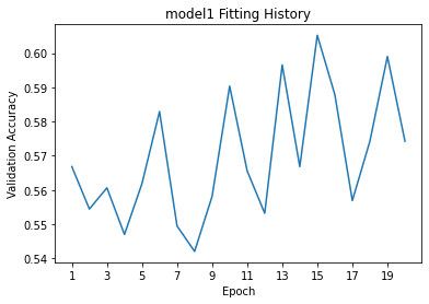
I played around with adding another Dense layer as well as different activation functions for Dense and Conv2D, but in this case simpler turned out to be better: I found the best results when I took out the extra Dense layer and with no specific activation function for most layers. Ultimately, the accuracy settled between 55% and 60% during fitting. This is admittedly not much better than baseline, but still a visible increase. There also seems to be mild overfitting, as the accuracy on the training data (~75%) is significantly higher than that of the validation data.
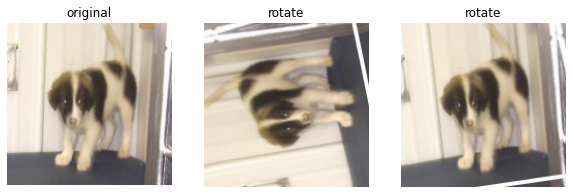
##Model 2 For our next model, we’ll be accounting for rigid transformations of images. After all, an image of a cat is still an image of a cat, whether it’s been flipped or rotated. It turns out that the layers modules contains RandomFlip() and RandomRotation() layers, so we can apply those to elements of the dataset. Let’s see an example of how they modify a sample image:
#take a sample image from train_dataset
sample_img = list(train_dataset)[0][0][0]
sample_img = sample_img.numpy().astype("uint8")
flip_layer = tf.keras.layers.RandomFlip()
rot_layer = tf.keras.layers.RandomRotation(factor=[0,1])
def plot_augmented(layer,title):
fig = plt.figure(figsize=(10,10))
for i in range(1,4):
ax = plt.subplot(1, 3, i)
if i == 1: #plots original image once
plt.imshow(sample_img)
plt.title("original")
else: #plots two modified images
plt.imshow(layer(sample_img).numpy().astype("uint8"))
plt.title(title)
plt.axis("off")
return fig
#make plots demonstrating flip and rotation layers
plot_augmented(flip_layer,"flip").show()
plot_augmented(rot_layer,"rotate").show()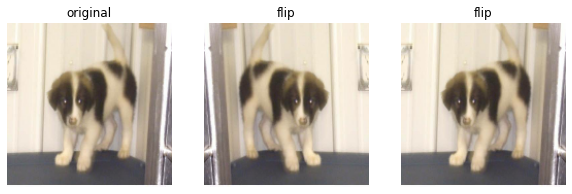
Now let’s append these layers to the beginning of our earlier model to create model2. We train this model and plot the results in the same way as earlier.
#create model2
model2 = tf.keras.models.Sequential([
    flip_layer,
    rot_layer,
    layers.Conv2D(2,3, input_shape=(160,160,3)),
    layers.MaxPooling2D(),
    layers.Dropout(rate=0.1),
    layers.Conv2D(2,3, input_shape=(80,80,3)),
    layers.MaxPooling2D(),
    layers.Dropout(rate=0.1),
    layers.Flatten(),
    layers.Dense(2, activation='softmax'),
])
#compile model
sce = tf.keras.losses.SparseCategoricalCrossentropy(from_logits=False)
model2.compile(optimizer='adam',
loss = sce,
metrics = ['accuracy'])#train model
history = model2.fit(train_dataset,
epochs=20,
validation_data=validation_dataset)Epoch 1/20WARNING:tensorflow:Using a while_loop for converting RngReadAndSkip cause there is no registered converter for this op.
WARNING:tensorflow:Using a while_loop for converting Bitcast cause there is no registered converter for this op.
WARNING:tensorflow:Using a while_loop for converting Bitcast cause there is no registered converter for this op.
WARNING:tensorflow:Using a while_loop for converting StatelessRandomUniformV2 cause there is no registered converter for this op.
WARNING:tensorflow:Using a while_loop for converting ImageProjectiveTransformV3 cause there is no registered converter for this op.
WARNING:tensorflow:Using a while_loop for converting RngReadAndSkip cause there is no registered converter for this op.
WARNING:tensorflow:Using a while_loop for converting Bitcast cause there is no registered converter for this op.
WARNING:tensorflow:Using a while_loop for converting Bitcast cause there is no registered converter for this op.
WARNING:tensorflow:Using a while_loop for converting StatelessRandomUniformV2 cause there is no registered converter for this op.
WARNING:tensorflow:Using a while_loop for converting ImageProjectiveTransformV3 cause there is no registered converter for this op.63/63 [==============================] - 12s 128ms/step - loss: 31.4179 - accuracy: 0.5215 - val_loss: 12.6689 - val_accuracy: 0.5210
Epoch 2/20
63/63 [==============================] - 9s 133ms/step - loss: 11.4337 - accuracy: 0.5115 - val_loss: 6.6900 - val_accuracy: 0.5297
Epoch 3/20
63/63 [==============================] - 9s 140ms/step - loss: 6.9246 - accuracy: 0.5220 - val_loss: 5.3629 - val_accuracy: 0.5681
Epoch 4/20
63/63 [==============================] - 8s 124ms/step - loss: 5.4743 - accuracy: 0.5115 - val_loss: 4.4900 - val_accuracy: 0.5631
Epoch 5/20
63/63 [==============================] - 8s 128ms/step - loss: 4.6692 - accuracy: 0.5385 - val_loss: 3.4300 - val_accuracy: 0.5755
Epoch 6/20
63/63 [==============================] - 8s 128ms/step - loss: 3.8303 - accuracy: 0.5285 - val_loss: 3.2468 - val_accuracy: 0.5396
Epoch 7/20
63/63 [==============================] - 8s 127ms/step - loss: 3.2185 - accuracy: 0.5230 - val_loss: 2.4864 - val_accuracy: 0.5557
Epoch 8/20
63/63 [==============================] - 7s 112ms/step - loss: 2.7107 - accuracy: 0.5405 - val_loss: 2.1628 - val_accuracy: 0.5755
Epoch 9/20
63/63 [==============================] - 8s 129ms/step - loss: 2.3468 - accuracy: 0.5420 - val_loss: 1.9320 - val_accuracy: 0.5829
Epoch 10/20
63/63 [==============================] - 8s 128ms/step - loss: 2.1449 - accuracy: 0.5205 - val_loss: 1.6054 - val_accuracy: 0.5681
Epoch 11/20
63/63 [==============================] - 7s 113ms/step - loss: 1.9699 - accuracy: 0.5190 - val_loss: 1.6049 - val_accuracy: 0.5644
Epoch 12/20
63/63 [==============================] - 8s 114ms/step - loss: 1.6947 - accuracy: 0.5240 - val_loss: 1.3322 - val_accuracy: 0.5705
Epoch 13/20
63/63 [==============================] - 8s 127ms/step - loss: 1.5412 - accuracy: 0.5330 - val_loss: 1.2898 - val_accuracy: 0.5644
Epoch 14/20
63/63 [==============================] - 8s 116ms/step - loss: 1.4501 - accuracy: 0.5320 - val_loss: 1.1926 - val_accuracy: 0.5730
Epoch 15/20
63/63 [==============================] - 8s 119ms/step - loss: 1.2969 - accuracy: 0.5545 - val_loss: 1.6691 - val_accuracy: 0.5631
Epoch 16/20
63/63 [==============================] - 8s 127ms/step - loss: 1.3607 - accuracy: 0.5100 - val_loss: 1.0632 - val_accuracy: 0.5730
Epoch 17/20
63/63 [==============================] - 7s 112ms/step - loss: 1.2319 - accuracy: 0.5470 - val_loss: 1.0500 - val_accuracy: 0.5396
Epoch 18/20
63/63 [==============================] - 8s 131ms/step - loss: 1.1507 - accuracy: 0.5450 - val_loss: 1.0001 - val_accuracy: 0.5582
Epoch 19/20
63/63 [==============================] - 9s 134ms/step - loss: 1.0252 - accuracy: 0.5525 - val_loss: 0.9651 - val_accuracy: 0.5619
Epoch 20/20
63/63 [==============================] - 7s 111ms/step - loss: 1.0521 - accuracy: 0.5300 - val_loss: 0.9494 - val_accuracy: 0.5606#plot model2 accuracies
model2_plot = plot_accuracies(history.history["val_accuracy"],"model2")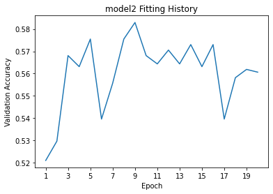
The validation accuracy is consistently between 55% and 58% for the most part. This is a few percent better compared to model1, and this time we do not observe overfitting, since the accuracy and validation accuracy are consistent.
##Model 3
Oftentimes, simple adjustments to the input data, e.g. normalizing the inputs, can improve efficiency and allow the model to use more energy training that it otherwise might have used to adjust weights. Tensorflow can handle this preprocessing for us with a layer.
#creates preprocessing layer
i = tf.keras.Input(shape=(160, 160, 3))
x = tf.keras.applications.mobilenet_v2.preprocess_input(i)
preprocessor = tf.keras.Model(inputs = [i], outputs = [x])
With this layer we create a third model that builds upon our second.
#create model
model3 = tf.keras.models.Sequential([
    preprocessor,
    flip_layer,
    rot_layer,
    layers.Conv2D(16,5),
    layers.MaxPooling2D((4,4)),
    layers.Conv2D(64,3),
    layers.MaxPooling2D((4,4)),
    layers.Dropout(rate=0.1),
    layers.Flatten(),
    layers.Dense(2, activation='softmax'),
])
WARNING:tensorflow:Using a while_loop for converting RngReadAndSkip cause there is no registered converter for this op.
WARNING:tensorflow:Using a while_loop for converting Bitcast cause there is no registered converter for this op.
WARNING:tensorflow:Using a while_loop for converting Bitcast cause there is no registered converter for this op.
WARNING:tensorflow:Using a while_loop for converting StatelessRandomUniformV2 cause there is no registered converter for this op.
WARNING:tensorflow:Using a while_loop for converting ImageProjectiveTransformV3 cause there is no registered converter for this op.#compile model
sce = tf.keras.losses.SparseCategoricalCrossentropy(from_logits=False)
model3.compile(optimizer='adam',
loss = sce,
metrics = ['accuracy'])#train model
history3 = model3.fit(train_dataset,
epochs=20,
validation_data=validation_dataset)Epoch 1/20WARNING:tensorflow:Using a while_loop for converting RngReadAndSkip cause there is no registered converter for this op.
WARNING:tensorflow:Using a while_loop for converting Bitcast cause there is no registered converter for this op.
WARNING:tensorflow:Using a while_loop for converting Bitcast cause there is no registered converter for this op.
WARNING:tensorflow:Using a while_loop for converting StatelessRandomUniformV2 cause there is no registered converter for this op.
WARNING:tensorflow:Using a while_loop for converting ImageProjectiveTransformV3 cause there is no registered converter for this op.
WARNING:tensorflow:Using a while_loop for converting RngReadAndSkip cause there is no registered converter for this op.
WARNING:tensorflow:Using a while_loop for converting Bitcast cause there is no registered converter for this op.
WARNING:tensorflow:Using a while_loop for converting Bitcast cause there is no registered converter for this op.
WARNING:tensorflow:Using a while_loop for converting StatelessRandomUniformV2 cause there is no registered converter for this op.
WARNING:tensorflow:Using a while_loop for converting ImageProjectiveTransformV3 cause there is no registered converter for this op.63/63 [==============================] - 12s 137ms/step - loss: 0.6994 - accuracy: 0.5465 - val_loss: 0.6339 - val_accuracy: 0.6597
Epoch 2/20
63/63 [==============================] - 8s 131ms/step - loss: 0.6604 - accuracy: 0.5820 - val_loss: 0.6207 - val_accuracy: 0.6522
Epoch 3/20
63/63 [==============================] - 8s 116ms/step - loss: 0.6351 - accuracy: 0.6395 - val_loss: 0.5910 - val_accuracy: 0.6881
Epoch 4/20
63/63 [==============================] - 7s 113ms/step - loss: 0.6257 - accuracy: 0.6585 - val_loss: 0.5843 - val_accuracy: 0.6980
Epoch 5/20
63/63 [==============================] - 8s 119ms/step - loss: 0.6158 - accuracy: 0.6725 - val_loss: 0.5912 - val_accuracy: 0.6832
Epoch 6/20
63/63 [==============================] - 8s 129ms/step - loss: 0.6148 - accuracy: 0.6640 - val_loss: 0.5603 - val_accuracy: 0.7463
Epoch 7/20
63/63 [==============================] - 7s 114ms/step - loss: 0.5973 - accuracy: 0.6870 - val_loss: 0.5579 - val_accuracy: 0.7389
Epoch 8/20
63/63 [==============================] - 8s 124ms/step - loss: 0.6031 - accuracy: 0.6775 - val_loss: 0.5869 - val_accuracy: 0.6819
Epoch 9/20
63/63 [==============================] - 8s 130ms/step - loss: 0.6075 - accuracy: 0.6740 - val_loss: 0.5651 - val_accuracy: 0.7030
Epoch 10/20
63/63 [==============================] - 8s 116ms/step - loss: 0.5908 - accuracy: 0.6855 - val_loss: 0.5488 - val_accuracy: 0.7426
Epoch 11/20
63/63 [==============================] - 8s 116ms/step - loss: 0.5874 - accuracy: 0.6920 - val_loss: 0.5443 - val_accuracy: 0.7413
Epoch 12/20
63/63 [==============================] - 8s 131ms/step - loss: 0.5767 - accuracy: 0.6980 - val_loss: 0.5599 - val_accuracy: 0.7054
Epoch 13/20
63/63 [==============================] - 8s 130ms/step - loss: 0.5919 - accuracy: 0.6935 - val_loss: 0.5940 - val_accuracy: 0.6955
Epoch 14/20
63/63 [==============================] - 7s 114ms/step - loss: 0.5890 - accuracy: 0.6880 - val_loss: 0.5414 - val_accuracy: 0.7290
Epoch 15/20
63/63 [==============================] - 8s 131ms/step - loss: 0.6049 - accuracy: 0.6720 - val_loss: 0.5863 - val_accuracy: 0.6955
Epoch 16/20
63/63 [==============================] - 8s 131ms/step - loss: 0.5934 - accuracy: 0.6980 - val_loss: 0.5490 - val_accuracy: 0.7475
Epoch 17/20
63/63 [==============================] - 8s 115ms/step - loss: 0.5830 - accuracy: 0.6965 - val_loss: 0.5590 - val_accuracy: 0.7191
Epoch 18/20
63/63 [==============================] - 8s 129ms/step - loss: 0.5825 - accuracy: 0.6810 - val_loss: 0.5385 - val_accuracy: 0.7389
Epoch 19/20
63/63 [==============================] - 8s 127ms/step - loss: 0.5863 - accuracy: 0.6945 - val_loss: 0.5470 - val_accuracy: 0.7277
Epoch 20/20
63/63 [==============================] - 7s 115ms/step - loss: 0.5776 - accuracy: 0.6960 - val_loss: 0.5168 - val_accuracy: 0.7525#plot model3 accuracies
model3_plot=plot_accuracies(history3.history["val_accuracy"],"model3")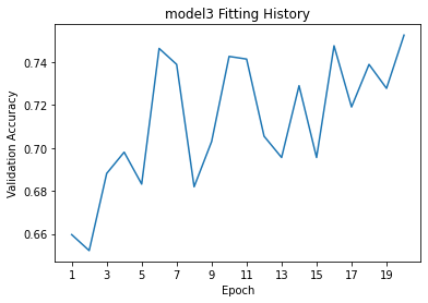
The validation accuracy settles between 70% and 75%, far better than for model1. Like with model2 we observe no significant overfitting, as the accuracy and validation accuracy are fairly consistent with each other. It should be noted that to reach a benchmark of at least 70% accuracy, we had to adjust both of our Conv2D() layers to use more output filters and use a different kernel size. By only adding the preprocessor layer to model2, we could only reach around 65% accuracy at most.
##Model 4
Finally, we implement transfer learning. For a task like this, there’s a high chance that there already exists a model that does something similar. And, as it turns out, there is one such model in Tensorflow. Transfer learning allows us to use that model as a layer in our own classification model.
#import base model
IMG_SHAPE = IMG_SIZE + (3,)
base_model = tf.keras.applications.MobileNetV2(input_shape=IMG_SHAPE,
                                               include_top=False,
                                               weights='imagenet')
base_model.trainable = False

#turn model into layer
i = tf.keras.Input(shape=IMG_SHAPE)
x = base_model(i, training = False)
base_model_layer = tf.keras.Model(inputs = [i], outputs = [x])
Downloading data from https://storage.googleapis.com/tensorflow/keras-applications/mobilenet_v2/mobilenet_v2_weights_tf_dim_ordering_tf_kernels_1.0_160_no_top.h5
9406464/9406464 [==============================] - 0s 0us/stepFor our final model, we’ll keep the preprocessing and data augmentation layers, but to keep it simple we replace the convolutions with base_model_layer. With luck, this model should be far more accurate than the other three!
#create model
model4 = tf.keras.models.Sequential([
    preprocessor,
    flip_layer,
    rot_layer,
    base_model_layer,
    layers.GlobalMaxPooling2D(),
    layers.Dense(2, activation='softmax'),
])
WARNING:tensorflow:Using a while_loop for converting RngReadAndSkip cause there is no registered converter for this op.
WARNING:tensorflow:Using a while_loop for converting Bitcast cause there is no registered converter for this op.
WARNING:tensorflow:Using a while_loop for converting Bitcast cause there is no registered converter for this op.
WARNING:tensorflow:Using a while_loop for converting StatelessRandomUniformV2 cause there is no registered converter for this op.
WARNING:tensorflow:Using a while_loop for converting ImageProjectiveTransformV3 cause there is no registered converter for this op.#compile model
sce = tf.keras.losses.SparseCategoricalCrossentropy(from_logits=False)
model4.compile(optimizer='adam',
loss = sce,
metrics = ['accuracy'])Let’s take a look at the layers of our model.
model4.summary()Model: "sequential_3"
_________________________________________________________________
Layer (type) Output Shape Param #
=================================================================
model (Functional) (None, 160, 160, 3) 0
random_flip (RandomFlip) (None, 160, 160, 3) 0
random_rotation (RandomRota (None, 160, 160, 3) 0
tion)
model_1 (Functional) (None, 5, 5, 1280) 2257984
global_max_pooling2d (Globa (None, 1280) 0
lMaxPooling2D)
dense_3 (Dense) (None, 2) 2562
=================================================================
Total params: 2,260,546
Trainable params: 2,562
Non-trainable params: 2,257,984
_________________________________________________________________We have to train 2562 parameters, but overall there are 2260546 parameters, most of which are coming from base_layer_model!
#train model
history4 = model4.fit(train_dataset,
epochs=20,
validation_data=validation_dataset)Epoch 1/20WARNING:tensorflow:Using a while_loop for converting RngReadAndSkip cause there is no registered converter for this op.
WARNING:tensorflow:Using a while_loop for converting Bitcast cause there is no registered converter for this op.
WARNING:tensorflow:Using a while_loop for converting Bitcast cause there is no registered converter for this op.
WARNING:tensorflow:Using a while_loop for converting StatelessRandomUniformV2 cause there is no registered converter for this op.
WARNING:tensorflow:Using a while_loop for converting ImageProjectiveTransformV3 cause there is no registered converter for this op.
WARNING:tensorflow:Using a while_loop for converting RngReadAndSkip cause there is no registered converter for this op.
WARNING:tensorflow:Using a while_loop for converting Bitcast cause there is no registered converter for this op.
WARNING:tensorflow:Using a while_loop for converting Bitcast cause there is no registered converter for this op.
WARNING:tensorflow:Using a while_loop for converting StatelessRandomUniformV2 cause there is no registered converter for this op.
WARNING:tensorflow:Using a while_loop for converting ImageProjectiveTransformV3 cause there is no registered converter for this op.63/63 [==============================] - 17s 166ms/step - loss: 0.6677 - accuracy: 0.8025 - val_loss: 0.1833 - val_accuracy: 0.9381
Epoch 2/20
63/63 [==============================] - 8s 130ms/step - loss: 0.3575 - accuracy: 0.8840 - val_loss: 0.1597 - val_accuracy: 0.9468
Epoch 3/20
63/63 [==============================] - 10s 140ms/step - loss: 0.3598 - accuracy: 0.8825 - val_loss: 0.2113 - val_accuracy: 0.9356
Epoch 4/20
63/63 [==============================] - 10s 148ms/step - loss: 0.3909 - accuracy: 0.8875 - val_loss: 0.1259 - val_accuracy: 0.9604
Epoch 5/20
63/63 [==============================] - 9s 146ms/step - loss: 0.3139 - accuracy: 0.9120 - val_loss: 0.1563 - val_accuracy: 0.9530
Epoch 6/20
63/63 [==============================] - 9s 145ms/step - loss: 0.3095 - accuracy: 0.9020 - val_loss: 0.0958 - val_accuracy: 0.9703
Epoch 7/20
63/63 [==============================] - 8s 130ms/step - loss: 0.2715 - accuracy: 0.9075 - val_loss: 0.1131 - val_accuracy: 0.9666
Epoch 8/20
63/63 [==============================] - 9s 141ms/step - loss: 0.3132 - accuracy: 0.8985 - val_loss: 0.1122 - val_accuracy: 0.9653
Epoch 9/20
63/63 [==============================] - 9s 145ms/step - loss: 0.2409 - accuracy: 0.9240 - val_loss: 0.1020 - val_accuracy: 0.9703
Epoch 10/20
63/63 [==============================] - 9s 144ms/step - loss: 0.2531 - accuracy: 0.9205 - val_loss: 0.1205 - val_accuracy: 0.9629
Epoch 11/20
63/63 [==============================] - 9s 132ms/step - loss: 0.2513 - accuracy: 0.9135 - val_loss: 0.1066 - val_accuracy: 0.9678
Epoch 12/20
63/63 [==============================] - 9s 147ms/step - loss: 0.2140 - accuracy: 0.9215 - val_loss: 0.1051 - val_accuracy: 0.9653
Epoch 13/20
63/63 [==============================] - 9s 144ms/step - loss: 0.2233 - accuracy: 0.9270 - val_loss: 0.1221 - val_accuracy: 0.9641
Epoch 14/20
63/63 [==============================] - 9s 144ms/step - loss: 0.2344 - accuracy: 0.9215 - val_loss: 0.0929 - val_accuracy: 0.9740
Epoch 15/20
63/63 [==============================] - 8s 127ms/step - loss: 0.1978 - accuracy: 0.9335 - val_loss: 0.0880 - val_accuracy: 0.9703
Epoch 16/20
63/63 [==============================] - 9s 145ms/step - loss: 0.2259 - accuracy: 0.9340 - val_loss: 0.1202 - val_accuracy: 0.9678
Epoch 17/20
63/63 [==============================] - 9s 143ms/step - loss: 0.2236 - accuracy: 0.9305 - val_loss: 0.1069 - val_accuracy: 0.9691
Epoch 18/20
63/63 [==============================] - 9s 142ms/step - loss: 0.2051 - accuracy: 0.9300 - val_loss: 0.1009 - val_accuracy: 0.9765
Epoch 19/20
63/63 [==============================] - 9s 134ms/step - loss: 0.2054 - accuracy: 0.9340 - val_loss: 0.1101 - val_accuracy: 0.9666
Epoch 20/20
63/63 [==============================] - 8s 131ms/step - loss: 0.1801 - accuracy: 0.9355 - val_loss: 0.1217 - val_accuracy: 0.9629#plot model4 accuracies
model4_plot = plot_accuracies(history4.history["val_accuracy"],"model4")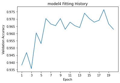
The validation accuracy of this model is consistently between 96% and 98%. This is significantly higher than any of our other models and shows no overfitting, since the testing accuracy is not significantly greater than the validation accuracy.
Now we can run this best-performing model on test_dataset and see how it does.
#evaluate model
model4.evaluate(test_dataset)
6/6 [==============================] - 1s 72ms/step - loss: 0.0470 - accuracy: 0.9896[0.046965230256319046, 0.9895833134651184]The accuracy of model4 is nearly 99%! The things that copying others’ work can do for you :)